40 modify legend labels excel 2013

Add and format a chart legend - support.microsoft.com Click the chart, and then click the Chart Design tab. Click Add Chart Element > Legend. To change the position of the legend, choose Right, Top, Left, or Bottom. To change the format of the legend, click More Legend Options, and then make the format changes that you want. Depending on the chart type, some options may not be available. How to Create a Quadrant Chart in Excel – Automate Excel We’re almost done. It’s time to add the data labels to the chart. Right-click any data marker (any dot) and click “Add Data Labels.” Step #10: Replace the default data labels with custom ones. Link the dots on the chart to the corresponding marketing channel names. To do that, right-click on any label and select “Format Data Labels.”

How to Create a Waterfall Chart in Excel - Automate Excel Right-click on the chart legend and choose “Delete” from the menu that pops up. Repeat the same process for the gridlines. Finally, change the chart title, and you can call it a day! How to Create a Waterfall Chart in Excel 2007, 2010, and 2013. This tutorial would end right here if the method shown above was compatible with all versions of ...

Modify legend labels excel 2013

Learn Excel 2013 - "Chart Legend Changes": Podcast #1693 Referring to Podcast #1408 where Bill showed us how to moved a Chart Legend, Bill begins today's podcast by describing and demonstrating not only the Moving ... Excel 2016: Charts - GCFGlobal.org Chart and layout style. After inserting a chart, there are several things you may want to change about the way your data is displayed. It's easy to edit a chart's layout and style from the Design tab.. Excel allows you to add chart elements—such as chart titles, legends, and data labels—to make your chart easier to read.To add a chart element, click the Add Chart Element command … Move and Align Chart Titles, Labels, Legends with the ... - Excel Campus Select the element in the chart you want to move (title, data labels, legend, plot area). On the add-in window press the "Move Selected Object with Arrow Keys" button. This is a toggle button and you want to press it down to turn on the arrow keys. Press any of the arrow keys on the keyboard to move the chart element.

Modify legend labels excel 2013. How to Add Axis Labels in Excel 2013 - YouTube How to Add Axis Labels in Excel 2013For more tips and tricks, be sure to check out is a tutorial on how to add axis labels in E... Excel 2013 legend entries in wrong order on stacked column charts Right-click on the legend and choose FORMAT LEGEND. In Excel 2013, change the LEGEND POSITION to LEFT or RIGHT. You may want to re-size the Legend Box again, but you'll find the entries in the right order. I've forgotten what the FORMAT LEGEND dialogue box looks like in earlier versions of Excel, but you just basically follow the same steps. How to rotate axis labels in chart in Excel? - ExtendOffice 1. Go to the chart and right click its axis labels you will rotate, and select the Format Axis from the context menu. 2. In the Format Axis pane in the right, click the Size & Properties button, click the Text direction box, and specify one direction from the drop down list. See screen shot below: Excel Chart Legend | How to Add and Format Chart Legend? - WallStreetMojo First, we need to go to the option "Chart Filters.". It helps to edit and modify the names and areas of the chart elements. Then click on "Select Data," as highlighted below in red. When we select the above option, a pop-up menu called the "Select Data Source" screen appears. In addition, there is an option of "Edit.".

Change marker size on legend - Excel Help Forum Re: Change marker size on legend. I'm sorry, it doesn't work on Mac. When you change de font for the last 'variable', all markers goes to their minimum size. The way I'm using now is: set the font size for legend larger and choose "Superscript" with "Offset: 1%". The size appearance of the font is reduced and similar of the rest in the chart. How to modify Chart legends in Excel 2013 - Stack Overflow 1 Answer Sorted by: 2 The words in the legend are sourced from the series name. You can point the series name to any cell in the spreadsheet. In the screenshot, the original series names were one, two and three. In the series definition, they got re-pointed to the cells that say blue, red and green. Modify chart legend entries - support.microsoft.com Edit legend entries in the Select Data Source dialog box Edit legend entries on the worksheet On the worksheet, click the cell that contains the name of the data series that appears as an entry in the chart legend. Type the new name, and then press ENTER. The new name automatically appears in the legend on the chart. Customize printing of a legend or title - support.microsoft.com In the Gantt chart view, click Gantt Chart Tools Format > Format > Bar Styles. To include a bar name in the printed legend, delete the asterisk in front of the name. And if you don't want to print a bar name, just add an asterisk in front the bar's name. Click File > Print and preview before printing.

Learn How to Access and Use 3D Maps in Excel - EDUCBA Map Labels – This labels all the locations, area, country on the map. Flat Map makes the 3D map into a 2D map in a beautiful way, worth trying it. Find Location – We can find any location by this all around the world. Refresh Data – If anything is updated in data, to make it visible on the map, use this. 2D Chart – It allows us to see a 3D chart in 2D. Legend – It shows the legends ... How to Change Data Label in Chart / Graph in MS Excel 2013 This video shows you how to change Data Label in Chart / Graph in MS Excel 2013.Excel Tips & Tricks : ... Chart axes, legend, data labels, trendline in Excel - Tech Funda To position the Data Labels in excel, select 'DESIGN > Add Chart Element > Data Labels > [appropriate command]'. For example, in below example, the data label has been positioned to Outside End. To format the Data Labels, select 'More Data Label Options...' and select approproate formatting from right side panel. Bringing Data Table on the chart How to Edit Legend Entries in Excel: 9 Steps (with Pictures) - wikiHow Select a legend entry in the "Legend entries (Series)" box. This box lists all the legend entries in your chart. Find the entry you want to edit here, and click on it to select it. 6 Click the Edit button. This will allow you to edit the selected entry's name and data values. On some versions of Excel, you won't see an Edit button.

Excel chart label: How to add, remove, position chart labels

Adding rich data labels to charts in Excel 2013 - microsoft.com You can do this by adjusting the zoom control on the bottom right corner of Excel's chrome. Then, select the value in the data label and hit the right-arrow key on your keyboard. The story behind the data in our example is that the temperature increased significantly on Wednesday and that appeared to help drive up business at the lemonade stand.

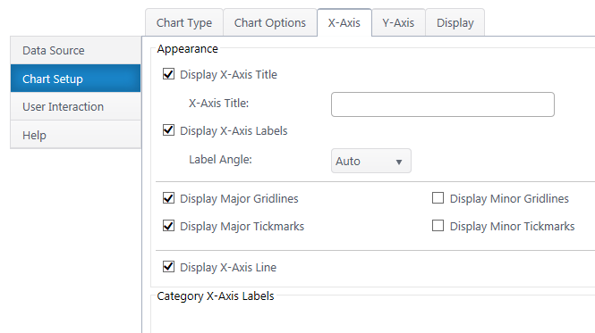
Chart Plus – Bamboo Solutions

Present your data in a scatter chart or a line chart 09.01.2007 · On the Layout tab, in the Labels group, click Legend, and then click the position that you want. For our line chart, we used Show Legend at Top . To plot one of the data series along a secondary vertical axis, click the data series for Rainfall, or select it from a list of chart elements ( Layout tab, Current Selection group, Chart Elements box).

How to do a running total in Excel (Cumulative Sum formula)

Learn How to Access and Use 3D Maps in Excel - EDUCBA Steps to Download 3D Maps in Excel 2013. 3D Maps are already inbuilt in Excel 2016. But for Excel 2013, we need to download and install packages as the add-in. This can be downloaded from the Microsoft website. For Excel 2013, 3D Maps are named as Power Maps. We can directly search this on the Microsoft website, as shown below. Downloading Step 1

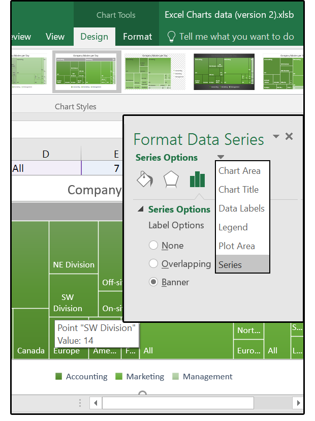
What to do with Excel 2016's new chart styles: Treemap, Sunburst, and Box & Whisker | PCWorld

Legends in Excel | How to Add legends in Excel Chart? - WallStreetMojo For changing the positioning of the legends in Excel 2013 and later versions, there is a small PLUS button on the right-hand side of the chart. If we click on that PLUS icon, we will see all the chart elements. Here we can change, enable, and disable all the chart elements.

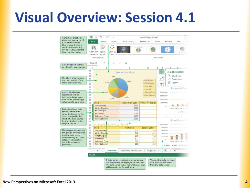
PPT - Excel Tutorial 4: Analyzing and Charting Financial Data PowerPoint Presentation - ID:1545005

Format and customize Excel 2013 charts quickly with the new Formatting ... The new Excel makes creating and customizing charts simpler and more intuitive. One part of the fluid new experience is the Formatting Task pane, which replaces the Format dialog box. The new Formatting Task pane is the single source for formatting--all of the different styling options are consolidated in one place. With this single task pane, you can modify not only charts, but also shapes ...

r - Multi-row x-axis labels in ggplot line chart - Stack Overflow

Waterfall Charts in Excel - A Beginner's Guide | GoSkills Excel will insert the chart on the spreadsheet which contains your source data. Our chart obviously needs some modification in order to be useful. Among other things, the steps below will show you how to: Add or remove data labels. Set a data point as a total or subtotal. Create or modify the chart title. Resize the chart. Add or remove axis ...

Share :