40 excel chart x axis labels

X Axis Labels Below Negative Values - Beat Excel! To do so, double-click on x axis labels. This will open "Format Axis" menu on left side of the screen. Make sure "Format Axis" menu is selected and if not, click on the area marked with dark green. This will open Format Axis menu. Then click on "Labels" as shown below. While in Labels menu, navigate to label position and select "Low". How to Add Axis Labels in Microsoft Excel - Appuals.com Click anywhere on the chart you want to add axis labels to. Click on the Chart Elements button (represented by a green + sign) next to the upper-right corner of the selected chart. Enable Axis Titles by checking the checkbox located directly beside the Axis Titles option.

Horizontal axis labels on a chart - Microsoft Community Fill a range of 12 cells with the months of the year. If you start with Jan or January, then fill down, Excel should automatically fill in the following names. Click on the chart. Click 'Select Data' on the 'Chart Design' tab of the ribbon. Click Edit under 'Horizontal (Category) Axis Labels'.

Excel chart x axis labels

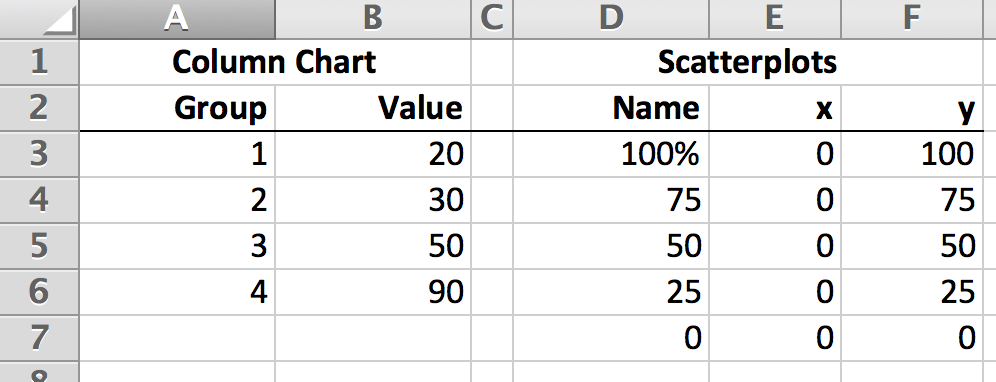
How to add text labels on Excel scatter chart axis Stepps to add text labels on Excel scatter chart axis 1. Firstly it is not straightforward. Excel scatter chart does not group data by text. Create a numerical representation for each category like this. By visualizing both numerical columns, it works as suspected. The scatter chart groups data points. 2. Secondly, create two additional columns. How to Change the X-Axis in Excel - Alphr Follow the steps to start changing the X-axis range: Open the Excel file with the chart you want to adjust. Right-click the X-axis in the chart you want to change. That will allow you to edit the... How to Add Axis Titles in a Microsoft Excel Chart - How-To Geek Select the chart and go to the Chart Design tab. Click the Add Chart Element drop-down arrow, move your cursor to Axis Titles, and deselect "Primary Horizontal," "Primary Vertical," or both. In Excel on Windows, you can also click the Chart Elements icon and uncheck the box for Axis Titles to remove them both.

Excel chart x axis labels. peltiertech.com › cusCustom Axis Labels and Gridlines in an Excel Chart Jul 23, 2013 · Adding Custom Axis Labels. We will add two series, whose data labels will replace the built-in axis labels. The horizontal axis dummy series (gray line and circle markers) uses the column of numbers (E2:E8) as X values and the column of zeros (F2:F8) as Y values. Excel Waterfall Chart: How to Create One That Doesn't Suck - Zebra BI Re-add vertical axis: Go to Design >> Add Chart Element >> Axes >> Primary Vertical "Break" vertical axis: right click on the vertical axis and click " Format Axis... ", then under Axis Options write " 35000 " under Bounds >> Minimum. Remove vertical axis: right click on the vertical axis and click " Delete " This is the chart we end up with: How To Change Y-Axis Values in Excel (2 Methods) Follow these steps to switch the placement of the Y and X-axis values in an Excel chart: 1. Select the chart Navigate to the chart containing your desired data. Click anywhere on the chart to allow editing and open the "Chart Settings" tab in the toolbar. Ensure that your cursor remains in the chart area to allow for editing. 2. Open "Select Data" Format Chart Axis in Excel - Axis Options Right-click on the Vertical Axis of this chart and select the "Format Axis" option from the shortcut menu. This will open up the format axis pane at the right of your excel interface. Thereafter, Axis options and Text options are the two sub panes of the format axis pane. Formatting Chart Axis in Excel - Axis Options : Sub Panes

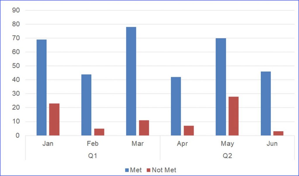
How to move Excel chart axis labels to the bottom or top - Data Cornering Move Excel chart axis labels to the bottom in 2 easy steps Select horizontal axis labels and press Ctrl + 1 to open the formatting pane. Open the Labels section and choose label position " Low ". Here is the result with Excel chart axis labels at the bottom. Now it is possible to clearly evaluate the dynamics of the series and see axis labels. › documents › excelHow to display text labels in the X-axis of scatter chart in ... Display text labels in X-axis of scatter chart. Actually, there is no way that can display text labels in the X-axis of scatter chart in Excel, but we can create a line chart and make it look like a scatter chart. 1. Select the data you use, and click Insert > Insert Line & Area Chart > Line with Markers to select a line chart. See screenshot: How to make a 3 Axis Graph using Excel? - GeeksforGeeks Make a three-axis graph in excel. To create a 3 axis graph follow the following steps: Step 1: Select table B3:E12. Then go to Insert Tab, and select the Scatter with Chart Lines and Marker Chart. Step 2: A Line chart with a primary axis will be created. Step 3: The primary axis of the chart will be Temperature, the secondary axis will be ... superuser.com › questions › 1195816Excel Chart not showing SOME X-axis labels - Super User Apr 05, 2017 · In Excel 2013, select the bar graph or line chart whose axis you're trying to fix. Right click on the chart, select "Format Chart Area..." from the pop up menu. A sidebar will appear on the right side of the screen. On the sidebar, click on "CHART OPTIONS" and select "Horizontal (Category) Axis" from the drop down menu.

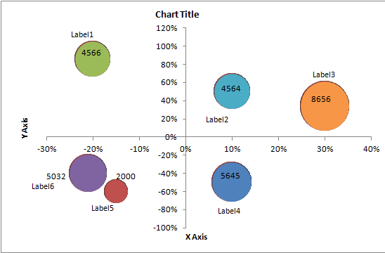
Date Axis in Excel Chart is wrong • AuditExcel.co.za If you right click on the horizontal axis and choose to Format Axis, you will see that under Axis Type it has 3 options being Automatic, text or date. As we have entered valid dates in the data the Automatic chooses dates and therefore you get the option in the second box. If Excel sees valid dates it will allow you to control the scale into ... Modifying Axis Scale Labels (Microsoft Excel) - tips Create your chart as you normally would. Double-click the axis you want to scale. You should see the Format Axis dialog box. (If double-clicking doesn't work, right-click the axis and choose Format Axis from the resulting Context menu.) Make sure the Scale tab is displayed. (See Figure 2.) Figure 2. The Scale tab of the Format Axis dialog box. How to Create and Customize a Pareto Chart in Microsoft Excel Go to the Insert tab and click the "Insert Statistical Chart" drop-down arrow. Select "Pareto" in the Histogram section of the menu. Remember, a Pareto chart is a sorted histogram chart. And just like that, a Pareto chart pops into your spreadsheet. You'll see your categories as the horizontal axis and your numbers as the vertical axis. Excel: How to Create a Bubble Chart with Labels - Statology Step 1: Enter the Data First, let's enter the following data into Excel that shows various attributes for 10 different basketball players: Step 2: Create the Bubble Chart Next, highlight the cells in the range B2:D11. Then click the Insert tab along the top ribbon and then click the Bubble Chart option within the Charts group:

How to Create a Chart with the Axis having Two Categories - ExcelNotes

Chart does not show correct horizontal axis labels Chart does not show correct horizontal axis labels. The horizontal axis labels on my chart are replaced by running numbers from 0 to 12. When I try to select data for that axis, the edit button is greyed out. I believe, the problem is that my labels are not years but half years (custom), so the system dies not recognize them as valid points in ...

34 X Axis Label Excel - Labels Database 2020

› excel-chart-verticalExcel Chart Vertical Axis Text Labels • My Online Training Hub Apr 14, 2015 · Now move the secondary vertical axis to the left hand side: right-click the axis (or double click if you have Excel 2010/13) > Format Axis > Axis Options: a. Major tick mark: None; b. Axis Labels: Low; c. Position on axis: On tick marks; d. Then go to the Line Color tab: No Line

How to Add a Third Y-Axis to a Scatter Chart | EngineerExcel

Axis.TickLabels property (Excel) | Microsoft Docs Returns a TickLabels object that represents the tick-mark labels for the specified axis. Read-only. Syntax expression. TickLabels expression A variable that represents an Axis object. Example This example sets the color of the tick-mark label font for the value axis on Chart1. VB Copy Charts ("Chart1").Axes (xlValue).TickLabels.Font.ColorIndex = 3

Bubble Charts - Negative Values in X-Axis and Multiple Bubble Colors - Chart (Obsolete) - UI for ...

8 Types of Excel Charts and Graphs and When to Use Them - MUO In the example above, if you included the name of the movies as the X-axis labels, you could identify which, of all of the movies listed, attracted a larger teen female audience. 7. Excel Surface Charts. These three-dimensional Excel chart types let you plot two sets of data points across several dimensions.

Changing Axis Labels in PowerPoint 2011 for Mac

› skip-dates-in-excelSkip Dates in Excel Chart Axis - My Online Training Hub Jan 28, 2015 · Right-click (Excel 2007) or double click (Excel 2010+) the axis to open the Format Axis dialog box > Axis Options > Text Axis: Now your chart skips the missing dates (see below). I’ve also changed the axis layout so you don’t have to turn your head to read them, which is always a nice touch.

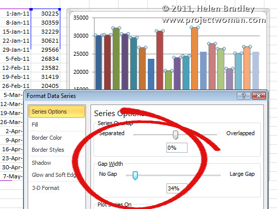
Help! My Excel Chart Columns are too Skinny « projectwoman.com

Two level axis in Excel chart not showing • AuditExcel.co.za In order to always see the second level, you need to tell Excel to always show all the items in the first level. You can easily do this by: Right clicking on the horizontal access and choosing Format Axis. Choose the Axis options (little column chart symbol) Click on the Labels dropdown. Change the 'Specify Interval Unit' to 1.

Custom Y-Axis Labels in Excel - Policy Viz

How to Show Percentage in Bar Chart in Excel (3 Handy Methods) - ExcelDemy Similar to the previous method, switch the rows and columns and choose the Years as the x-axis labels. Next, go to Chart Element > Data Labels. Following, double-click to select the label and select the cell reference corresponding to that bar. In the picture below, we chose the C13 cell. Finally, you should get the following results.

Excel isn't showing some of my Horizontal (Category) Axis Labels - Super User

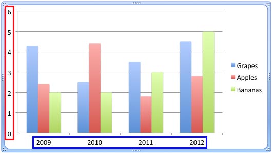
Two-Level Axis Labels (Microsoft Excel) - ExcelTips (ribbon) Excel automatically recognizes that you have two rows being used for the X-axis labels, and formats the chart correctly. Since the X-axis labels appear beneath the chart data, the order of the label rows is reversed—exactly as mentioned at the first of this tip. (See Figure 1.) Figure 1. Two-level axis labels are created automatically by Excel.

Share :