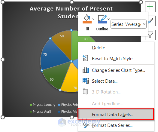
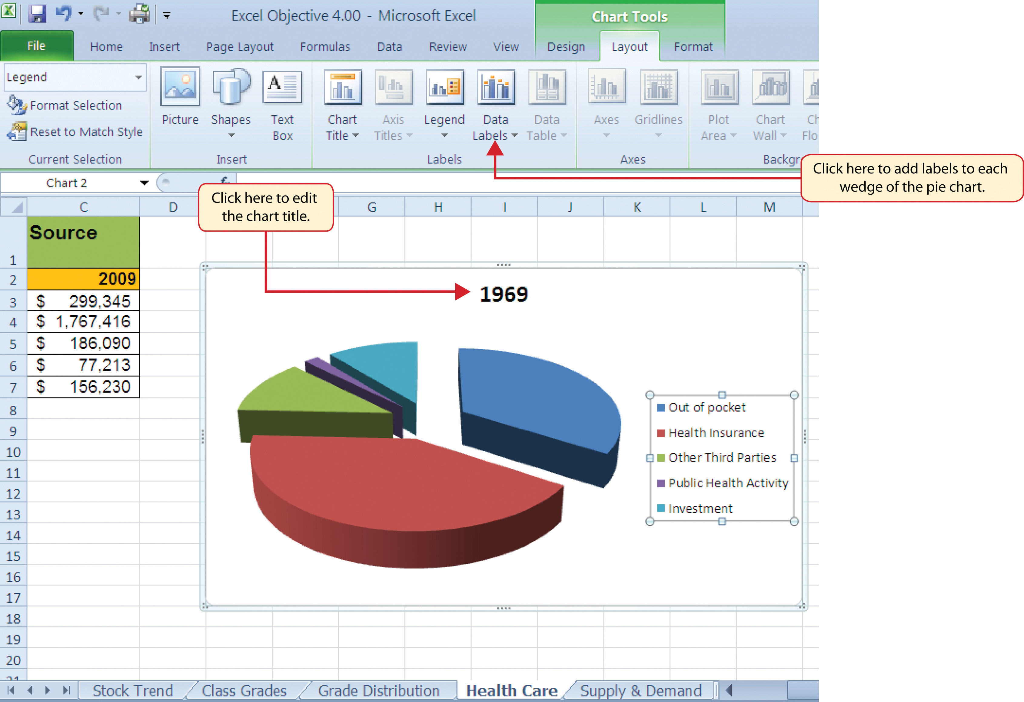
43 use the format data labels task pane to display category name and percentage data labels

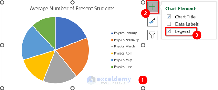
UsetheFormatDataLabelstaskpanetodisplay | Course Hero Use the Format Data Labels task pane to display Percentage data labels and remove the Value data labels. Close the task pane. Apply 18 point size to the data labels. a. Click green plus data labels center click green plus double click in chart label contains click percentage click values check box click close click home font 18 9. How to: Display and Format Data Labels - DevExpress In particular, set the DataLabelBase.ShowCategoryName and DataLabelBase.ShowPercent properties to true to display the category name and percentage value in a data label at the same time. To separate these items, assign a new line character to the DataLabelBase.Separator property, so the percentage value will be automatically wrapped to a new line.

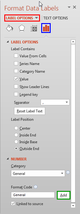
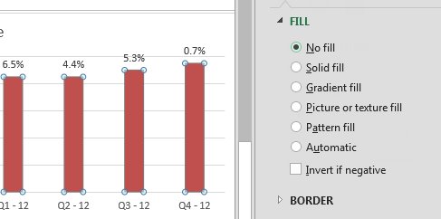
How to show data label in "percentage" instead of - Microsoft Community Select Format Data Labels Select Number in the left column Select Percentage in the popup options In the Format code field set the number of decimal places required and click Add. (Or if the table data in in percentage format then you can select Link to source.) Click OK Regards, OssieMac Report abuse 8 people found this reply helpful ·

Use the format data labels task pane to display category name and percentage data labels

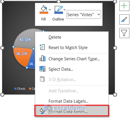
New User Guide — openmediavault 5.x.y documentation - Read … New User Guide¶. This document can be converted to a PDF file, at the bottom left side corner of this page. Click the drop down arrow next to Read the Doc’s v: 5.x. Google Translate kann Wiki-Dokumente in Ihre Sprache übersetzen. Fügen Sie die Wiki-URL in das linke Fenster ein und öffnen Sie den übersetzten Link rechts. 4.2 Formatting Charts - Beginning Excel, First Edition On the Design tab select the Add Chart Element button, then Data Labels, then Outside End (see Figure 4.36.) Click on one of the Data Labels. Note that all of the data labels for that data series are selected. Using the Home ribbon, change the font to Arial, Bold, size 9. Click on one of the data labels for the other data series. How to make a Gantt chart in Excel - Ablebits.com 30/09/2022 · Remove excess white space between the bars. Compacting the task bars will make your Gantt graph look even better. Click any of the orange bars to get them all selected, right click and select Format Data Series.; In the Format Data Series dialog, set Separated to 100% and Gap Width to 0% (or close to 0%).; And here is the result of our efforts - a simple but nice …

Use the format data labels task pane to display category name and percentage data labels. Change the format of data labels in a chart To get there, after adding your data labels, select the data label to format, and then click Chart Elements > Data Labels > More Options. To go to the appropriate area, click one of the four icons ( Fill & Line, Effects, Size & Properties ( Layout & Properties in Outlook or Word), or Label Options) shown here. Excel 2016 Tutorial Formatting Data Labels Microsoft Training ... - YouTube FREE Course! Click: about Formatting Data Labels in Microsoft Excel at . A clip from Mastering Excel M... cs 385 exam 3 Flashcards | Quizlet data tab, subtotal, click at each change in: select area, unselect replace current subtotals, click ok Collapse the table to show the grand totals only. click 1 at top left corner Expand the table to show the grand and discipline totals. click 2 at top left corner Use the Auto Outline feature to group the columns. Create timeline in powerpoint from excel data racism articles a b c Highlight all of your rows of data in your "Chart Data" tab and then click "Recommended Charts" within the "Insert" ribbon. Excel will suggest some charts for you to use. 4. Select your data.Now that you have that blank box inserted in your "Dashboard" tab of your workbook, it's time to pull some data in. Hello there, I have been experimenting with creating …

(Get Answer) - Share Format Data Labels Display Outside End data labels ... Share Format Data Labels Display Outside End data labels on the pie chart. Close the Chart Elements menu. Use the Format Data Labels task pane to display Percentage data labels and remove the Value data labels. Close the task pane. Excel chapter 3: grader project | Management homework help - SweetStudy Add Percent and Category Name data labels and choose Outside End position for the labels. Change the data labels font size to 10. 810You want to emphasize the Education & Training slice by exploding it. Explode the Education & Training slice by 12%. 211Add the Light Gradient - Accent 2 fill color to the chart area. Release Notes for Beta Channel - Office release notes 11/06/2020 · We fixed an issue that caused the Display Name and Trendline Name for a chart data series to be unable to be edited in the Chart Settings pane. Excel . We fixed an issue where the text fields in the custom filter dialog would autocomplete when you start typing a value. We fixed an issue where, when typing double-byte characters and there are two suggestions, one … Exp19_excel_ch03_cap_gym | Computer Science homework help You decide to format the pie chart with data labels and remove the legend because there are too many categories for the legend to be effective. Display the Expenses sheet and remove the legend. Add Percent and Category Name data labels and choose Outside End position for the labels. Change the data labels font size to 10.

Format Data Labels in Excel- Instructions - TeachUcomp, Inc. To format data labels in Excel, choose the set of data labels to format. To do this, click the "Format" tab within the "Chart Tools" contextual tab in the Ribbon. Then select the data labels to format from the "Chart Elements" drop-down in the "Current Selection" button group. Solved 5 3 5 5 You want to create a clustered | Chegg.com You decide to format the pie chart with data labels and remove the legend because there are too many categories for the legend to be effective. Display the Expenses sheet and remove the legend. Add Percent and Category Name data labels and choose Outside End position for the labels. Change the data labels font size to 10. 8: 10 How to use data labels - Exceljet When first enabled, data labels will show only values, but the Label Options area in the format task pane offers many other settings. You can set data labels to show the category name, the series name, and even values from cells. In this case for example, I can display comments from column E using the "value from cells" option. Advanced Excels With EPPlus - CodeProject 23/05/2018 · The returned instance of ExcelPieChartSerie lets you to change the appearance of the data labels ... will sum up to the sub category percentage of the total revenues. We start by adding the Revenue column as a pivot data column, but we also set the display format to percentage format 0.00%. C# // values: % Revenue ExcelPivotTableDataField …

How to Use Cell Values for Excel Chart Labels

Excel 3-D Pie charts - Microsoft Excel 2016 - OfficeToolTips 2. On the Insert tab, in the Charts group, choose the Pie button: Choose 3-D Pie. 3. Right-click in the chart area, then select Add Data Labels and click Add Data Labels in the popup menu: 4. Click in one of the labels to select all of them, then right-click and select Format Data Labels... in the popup menu: 5.

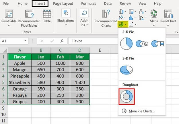
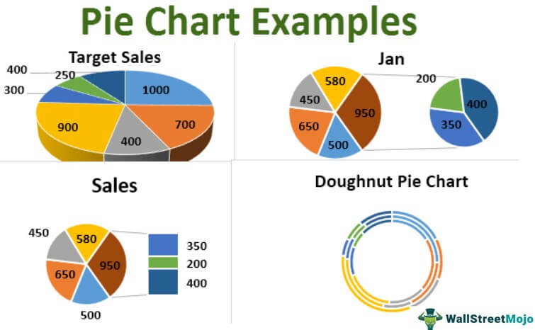
Pie Charts in Excel - How to Make with Step by Step Examples

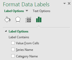
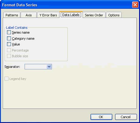
A data label is descriptive text that shows that - Course Hero To format the data labels - Double click a data label to open the Format Data Labels task pane. Click the Label Options Icon. Click Label Options to customize the labels, and complete any of the following steps: Select the Label Contains options. The default is Value, but you might want to display additional label contents, such as Category Name.

How to Make a Pie Chart in Excel (5 Suitable Examples)

Filtering charts in Excel | Microsoft 365 Blog Select the chart, then click the Filter icon to expose the filter pane. From here, you can filter both series and categories directly in the chart. For example, hover over Fruit Pear and see how the category is highlighted. To get the same view we created in our earlier chart, we'll hide the Cost/lb column. Under Series, uncheck Cost/lb, and ...

Change the format of data labels in a chart

How to create a chart with both percentage and value in Excel? In the Format Data Labels pane, please check Category Name option, and uncheck Value option from the Label Options, and then, you will get all percentages and values are displayed in the chart, see screenshot: 15.

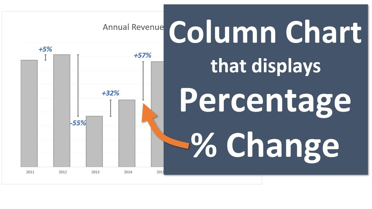
Column Chart That Displays Percentage Change or Variance ...

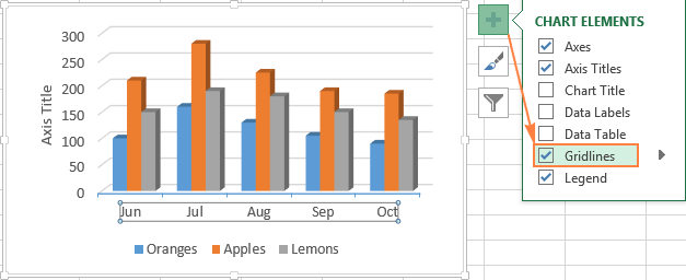
Excel charts: add title, customize chart axis, legend and data labels Click anywhere within your Excel chart, then click the Chart Elements button and check the Axis Titles box. If you want to display the title only for one axis, either horizontal or vertical, click the arrow next to Axis Titles and clear one of the boxes: Click the axis title box on the chart, and type the text.

Pie Charts in Excel - How to Make with Step by Step Examples

Work Distribution Report with Hours and Percentages Now right-click the doughnut and select Format Data Labels; then select Percentage, Category Name, Value, Legend Key, Show Leader Lines in the Format Data Labels pane (LABEL OPTIONS), and also ...

Excel charts: add title, customize chart axis, legend and ...

Excel Chapter 3 Flashcards | Quizlet 1. select the chart and click the design tab 2. click change chart type in the type group to open the change chart type dialogue box (which is similar to the insert chart dialogue box) 3. Click the all charts tab within the dialogue box 4. click a chart type on the left side of the dialogue box

Creating a Pie Chart: IU Only: Files: Excel 2016: Charts and ...

How to work on spreadsheet document using the information given Set the pie explosion percentage at 10%. Close the task pane. Click the chart object border to deselect the Atlanta slice. Add and format chart elements in a pie chart. Click the Chart Elements button in the top-right corner of the chart. Select the Data Labels box. Click the Data Labels arrow to open its submenu and choose More Options. If ...

How to insert data labels to a Pie chart in Excel 2013

Display the percentage data labels on the active chart. - YouTube Display the percentage data labels on the active chart.Want more? Then download our TEST4U demo from TEST4U provides an innovat...

Ultimate Guide to Creating Charts in Excel [2022] - onsite ...

How to show percentages on three different charts in Excel To convert the calculated decimal values to percentages, right-click on the selected cells and click Format Cells. Alternatively, press CTRL+1 on the keyboard to open the Format Cells dialogue box. 3. In the Format Cells dialogue box, make sure that the Number tab is selected and in the Category list select Percentage.

Change the format of data labels in a chart

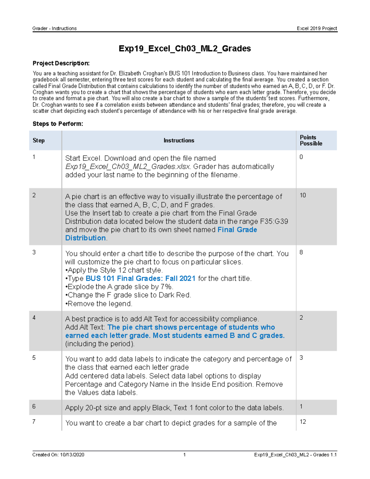
Solved step by step instruction 2 A pie chart is an | Chegg.com Use the Insert tab to create a pie chart from the Question: step by step instruction 2 A pie chart is an effective way to visually illustrate the percentage of the class that earned A, B, C, D, and F grades. Use the Insert tab to create a pie chart from the This problem has been solved! See the answer step by step instruction Expert Answer

How to show the percentage on stacked colum/bar chart in ...

Add or remove data labels in a chart - support.microsoft.com Right-click the data series or data label to display more data for, and then click Format Data Labels. Click Label Options and under Label Contains, select the Values From Cells checkbox. When the Data Label Range dialog box appears, go back to the spreadsheet and select the range for which you want the cell values to display as data labels.

Display Customized Data Labels on Charts & Graphs

Microsoft 365 Roadmap | Microsoft 365 You can create PivotTables in Excel that are connected to datasets stored in Power BI with a few clicks. Doing this allows you get the best of both PivotTables and Power BI. Calculate, summarize, and analyze your data with PivotTables from your secure Power BI datasets. More info. Feature ID: 63806; Added to Roadmap: 05/21/2020; Last Modified ...

How to show percentages on three different charts in Excel ...

Sharing Tips and tricks about Microsoft Office Outlook Kutools for Outlook: It includes 100+ handy features and functions to free you from time-comsuming operations in Outlook 2019-2010. Free Trial. Office Tab: Bringing a handy tabbed interface in your Microsoft Office 2019-2003. Free Trial

How to create a chart with both percentage and value in Excel?

(PDF) Advanced excel tutorial | Adeel Zaidi - Academia.edu 25/10/1983 · Alternatively, you can also click on More Options available in the Data Labels options to display the Format Data Label Task Pane. The Format Data Label Task Pane appears. There are many options available for formatting of the Data Labels in the Format Data Labels Task Pane. Make sure that only one Data Label is selected while formatting. 29 …

Label Options for Chart Data Labels in PowerPoint 2013 for ...

Assignment Paper - Custom Paper Writings Service You decide to format the pie chart with data labels and remove the legend because there are too many categories for the legend to be effective. Display the Expenses sheet and remove the legend. Add Percent and Category Name data labels and choose Outside End position for the labels. Change the data labels font size to 10. 8. 10

Change the format of data labels in a chart

How do you format data series in Excel? - FAQ-ALL Select the decimal number cells, and then click Home > % to change the decimal numbers to percentage format . 7. Then go to the stacked column, and select the label you want to show as percentage , then type = in the formula bar and select percentage cell, and press Enter key. How to format data series independently in Excel

Add or remove data labels in a chart

How to make a Gantt chart in Excel - Ablebits.com 30/09/2022 · Remove excess white space between the bars. Compacting the task bars will make your Gantt graph look even better. Click any of the orange bars to get them all selected, right click and select Format Data Series.; In the Format Data Series dialog, set Separated to 100% and Gap Width to 0% (or close to 0%).; And here is the result of our efforts - a simple but nice …

How to show percentages on three different charts in Excel ...

4.2 Formatting Charts - Beginning Excel, First Edition On the Design tab select the Add Chart Element button, then Data Labels, then Outside End (see Figure 4.36.) Click on one of the Data Labels. Note that all of the data labels for that data series are selected. Using the Home ribbon, change the font to Arial, Bold, size 9. Click on one of the data labels for the other data series.